2. Example application
An example application app.py can be found in the examples directory.
The creation of a FieldAnimation image is straightforward: just instantiate
the fieldanimation.FieldAnimation class passing the vector field
array and call its draw method within the main rendering loop.
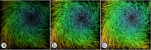
The visualization application shown above
depends on two OpenGL packages:
for rendering the OpenGL image created by FieldAnimation in a windowing system.
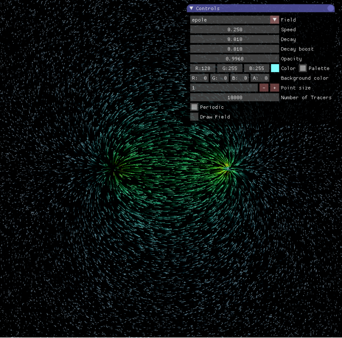
The interactive GUI in this figure allows to modify the visualization parameters that FieldAnimation embeds as instance attributes:
# Default values of the class attributes
FieldAnimation.speedFactor = 0.25
FieldAnimation.decay = 0.003
FieldAnimation.decayBoost = 0.01
FieldAnimation.fadeOpacity = 0.996
FieldAnimation.color = (0.5 , 1.0 , 1.0)
FieldAnimation.palette = True
FieldAnimation.pointSize = 1.0
FieldAnimation.tracersCount = 10000
FieldAnimation.periodic = True
FieldAnimation.drawField = False
Here is a detailed description of the controls that appear in the GUI:
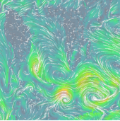
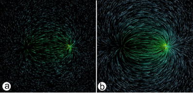
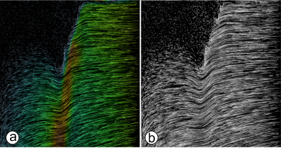
- Field: select one of the available vector fields implemented.
- Speed: set the length of the field pathlines i.e. the speed of the particles: the higher the value the longer the particle trace length.
- Decay: set the life span of a particle.
- Decay boost: increase points density in low intensity field areas.
- Opacity: set opacity of the particles over the background image.
- Color: set color of the particles according to the the field strength trough a cubehelix based color map.
- Palette: set color of the particles to a constant value.
- Point size: set the size of the animated particles (in pixels).
- Number of Tracers: set the number of the moving particles.
- Periodic: if checked points that move outside the border of the rendering window will enter from the opposite one.
- Draw Field: Draw the field modulus as a background image. In this example application the field modulus is rendered trough a cubehelix color map.